Road defects from the sky: from a benchmark to a map in QGIS
Published · 9 min read
My master's thesis at NUST MISIS asked a practical question: can a drone and an object detector replace the person who walks a road with a clipboard? The work produced two papers, a small desktop tool and one lesson I keep coming back to: a model that scores well on a benchmark has done maybe half the job.
This post covers what I built, which training choices actually moved the numbers, and what happened when the model met survey imagery it had never seen.
The problem
Cracks, potholes and alligator cracking are the early signs of a road failing. Fixed early, they are cheap. Left alone, traffic and weather turn them into repairs that cost far more. Yet most road surveys are still done by hand: an engineer walks or drives a section and writes down what they see. It is slow, it disrupts traffic, and two engineers rarely log the same road the same way.
A drone covers kilometres of road in minutes. Stitched into an orthophoto, a single georeferenced image of the whole area, the imagery is sharp enough to show cracks a few millimetres wide. Add a trained detector and you have the start of an automated survey.
Papers on this topic usually stop at a benchmark score. I wanted three things they tend to skip:
- Which training choices matter. Most papers report one tuned configuration. I wanted to know which change bought how much.
- What happens on real survey imagery. Benchmark images and survey orthophotos are taken at different heights, so the same crack looks a different size to the model.
- Output an engineer can use. Bounding boxes in pixel coordinates are useless to someone planning repairs. They need positions on a map.
How it fits together
The whole project in one picture: data in, four stages, a map out. The rest of this post walks through each stage.
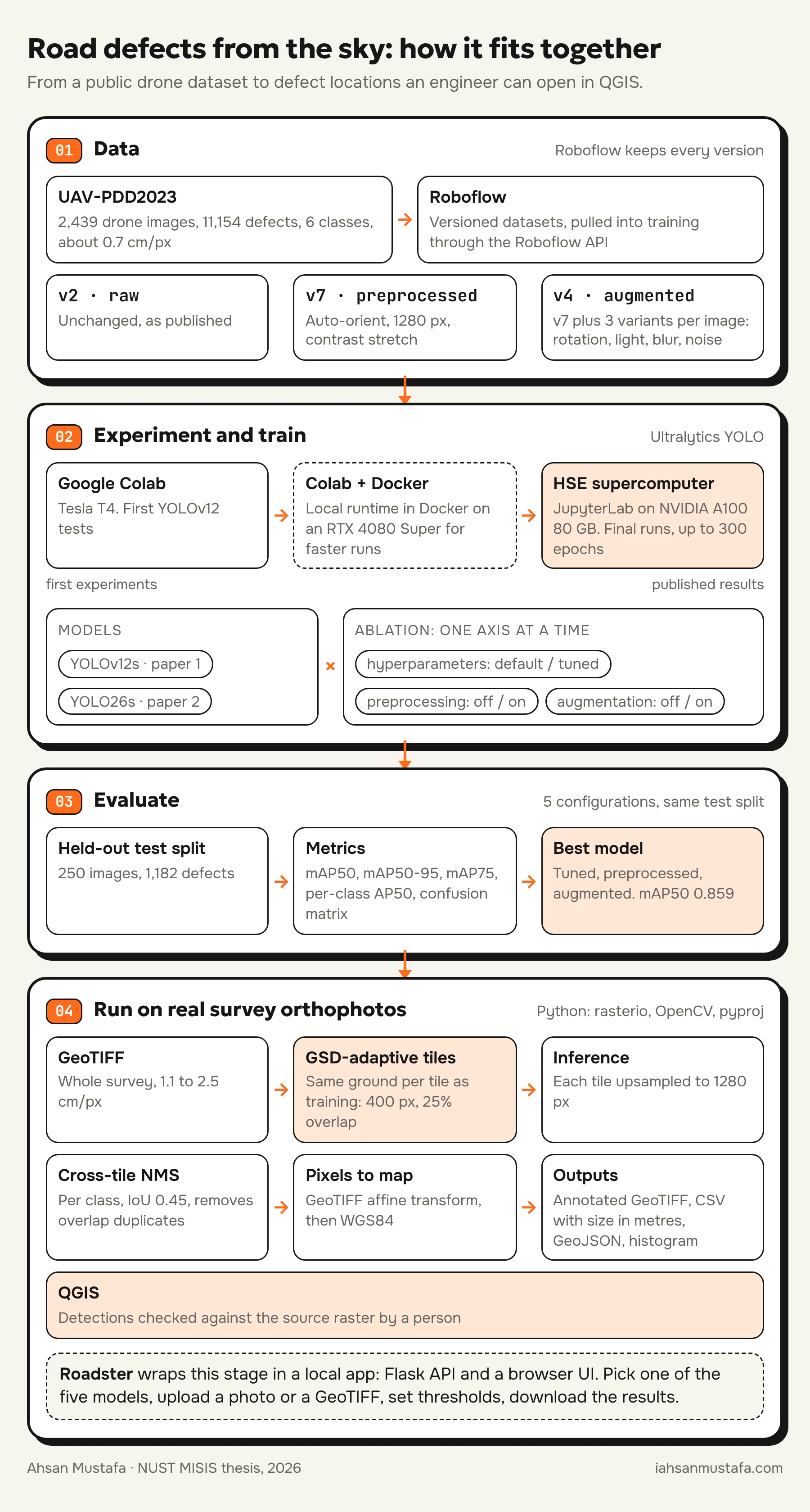
The compute grew with the project. The first YOLOv12 tests ran in Google Colab on a free T4. To iterate faster I then ran Colab against a local runtime in Docker on my own RTX 4080 Super. The published results came from JupyterLab on HSE University's supercomputer, on an NVIDIA A100 with 80 GB of memory. That is what made 1280 px inputs and 300-epoch runs practical.
Roboflow sat in the middle as the dataset store. Every preprocessing and augmentation choice became its own dataset version, and each training run pulled an exact version through the Roboflow API. That is what made the ablation honest: when two runs differ, I know which version each one saw.
The data
Everything was trained on UAV-PDD2023, a public benchmark of drone images of roads in China: 2,439 images, 11,154 labelled defects, six classes (alligator crack, longitudinal crack, oblique crack, transverse crack, pothole and repair patch).
| Split | Images | Defects |
|---|---|---|
| Train | 1,709 | 7,689 |
| Validation | 480 | 2,283 |
| Test | 250 | 1,182 |
The classes are badly imbalanced. Longitudinal and transverse cracks have thousands of examples each; potholes and oblique cracks together have fewer than 1,500. That imbalance shows up in every result below.
First pass: YOLOv12 and a colour question
The first paper, in Light & Engineering, compared two YOLOv12s setups: a baseline at 640 px with no augmentation, and an improved one at 1280 px with preprocessing and augmentation. The improved model reached mAP50-95 of 0.448 against the baseline's 0.134.
It also asked a question that matters for real drones: cameras differ. What if the survey camera only gives you one colour channel? We ran the RGB-trained models on single-channel versions of images from a separate drone flight, without retraining. More than 90% of the defects found in RGB were also found in a single channel. The better-trained model was also the more stable one: its total detection count moved by 10 to 20% between channels, against 15 to 25% for the baseline.
That paper answered "does it work". It didn't answer "why does it work", which is what the second one was for.
The ablation: what actually moved the numbers
For the second paper, now in press in Moscow University Physics Bulletin and presented at DLCP 2026, I switched to YOLO26s and changed one thing at a time along three axes:
- Hyperparameters: Ultralytics defaults (DP), or a tuned set (BP) with 1280 px input and 300 epochs.
- Preprocessing: none (NPP), or auto-orientation, 1280 × 1280 resize and contrast stretching (BPP).
- Augmentation: none (NAUG), or three augmented copies of each training image with small rotations, brightness, saturation, blur and noise (BAUG).
Five configurations, all scored on the same held-out test split:
| Configuration | mAP50 | mAP50-95 | mAP75 |
|---|---|---|---|
| Baseline (DP, NPP, NAUG) | 0.547 | 0.271 | 0.218 |
| DP, BPP, NAUG | 0.645 | 0.350 | 0.347 |
| BP, NPP, NAUG | 0.763 | 0.477 | 0.508 |
| DP, BPP, BAUG | 0.769 | 0.480 | 0.539 |
| BP, BPP, BAUG | 0.859 | 0.631 | 0.740 |
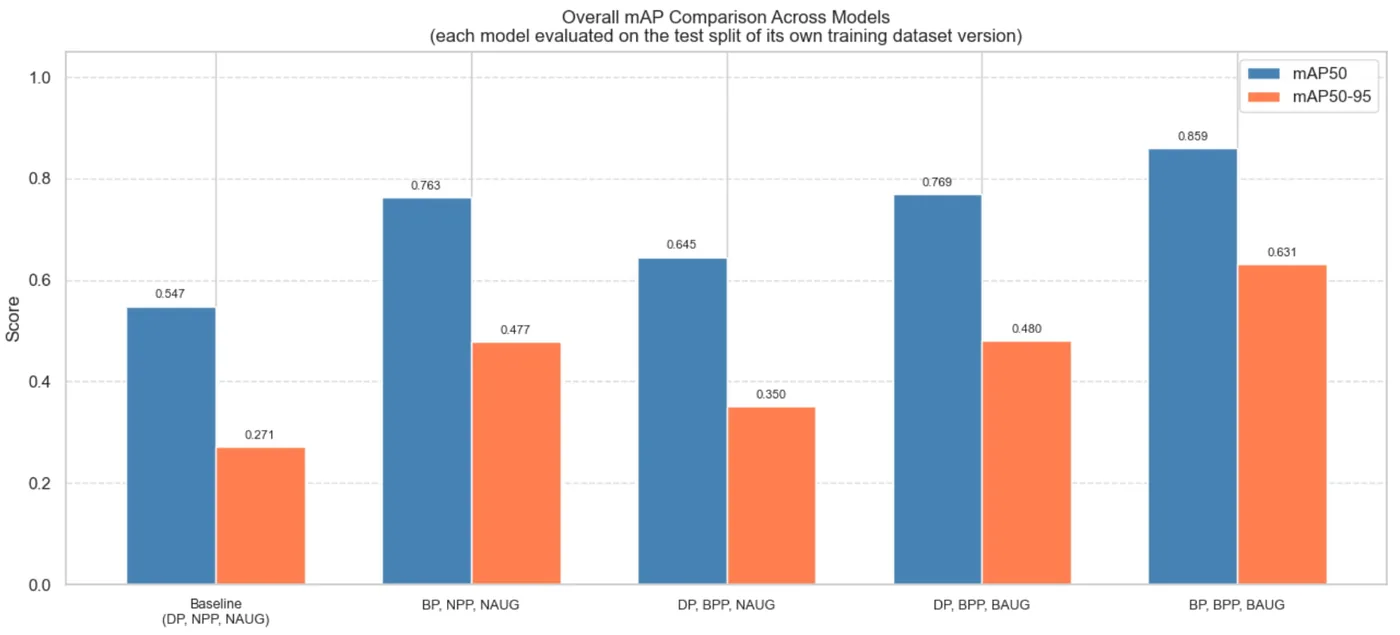
The full combination improves mAP50 by 57% and mAP50-95 by 133% over the defaults. The tuned hyperparameters alone get more than two thirds of the way there.
There is a caveat I want to be upfront about, and the paper states it too. The tuned hyperparameters change two things at once: input resolution and training length. So I can say the bundle is the biggest single win, but not that resolution alone is. The per-class results point strongly at resolution, but "points strongly" is not "isolated". Separating the two is the first experiment I'd run next.
Per class
| Class | Baseline AP50 | Best AP50 | Gain |
|---|---|---|---|
| Alligator crack | 0.623 | 0.949 | +0.326 |
| Longitudinal crack | 0.625 | 0.901 | +0.276 |
| Oblique crack | 0.362 | 0.797 | +0.435 |
| Pothole | 0.446 | 0.774 | +0.328 |
| Repair | 0.624 | 0.877 | +0.253 |
| Transverse crack | 0.605 | 0.857 | +0.252 |
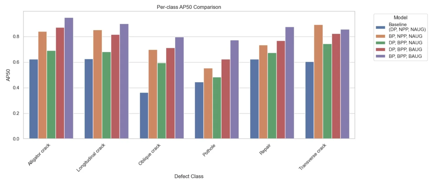
Two classes tell the story:
- Oblique cracks gained the most. At 640 px a diagonal crack is a few pixels wide and looks a lot like a longitudinal one. At 1280 px its angle survives and the model can tell them apart. That is a resolution problem, not a hard-to-learn class.
- Potholes gained mostly from augmentation. They are the rarest class, and three varied copies of each example helped more than extra pixels did. They are still the weakest class, and on validation images the model often gives them a confidence between 0.4 and 0.7.
From benchmark to a real road
This is the part I find most interesting, and the part benchmark papers skip.
The scale problem
Ground sampling distance (GSD) is how much ground one pixel covers. UAV-PDD2023 was shot low, at about 0.7 cm per pixel. Survey orthophotos are flown higher and land around 1 to 3 cm per pixel.
So a 1280 px tile from a survey at 2.5 cm/px covers 32 m of road, while the model learned on tiles covering about 9 m. A pothole that was 50 pixels across in training shrinks to about 14 pixels, too small to detect reliably. Feed the model the survey the naive way and it is looking at a different world.
Tile by ground, not by pixels
The fix is to choose the tile size so each tile covers the same ground the model saw in training:
# 1280 px at the training GSD covers ~9 m of road.
# Pick the field tile so it covers the same distance.
tile_px = round(1280 * gsd_train / gsd_field)   # 1280 * 0.7 / 2.5 ≈ 358, rounded up to 400
stride = int(tile_px * 0.75)                    # 25% overlap so no defect is cut in every tile
A 400 px tile at 2.5 cm/px covers 10 m. Ultralytics upsamples it to 1280 px before inference, so the model sees a crack at roughly the size it learned. The 25% overlap means a defect on one tile's edge sits whole inside a neighbour.
Overlap creates duplicates, so after inference every box goes back into full-image coordinates and I run per-class non-maximum suppression across the whole orthophoto (IoU 0.45). Then each box is pushed through the GeoTIFF's affine transform with rasterio, and converted to WGS84 with pyproj when the raster is in UTM. Width and height in metres fall out of the GSD.
For each orthophoto the pipeline writes:
- an annotated GeoTIFF with colour-coded boxes,
- a CSV with class, confidence, latitude, longitude, width, height and area in m²,
- a GeoJSON file that opens straight in QGIS,
- a histogram of confidence scores.
Three real orthophotos
I tested on three orthophotos from a different region, flown higher than the training data, and never seen in training.
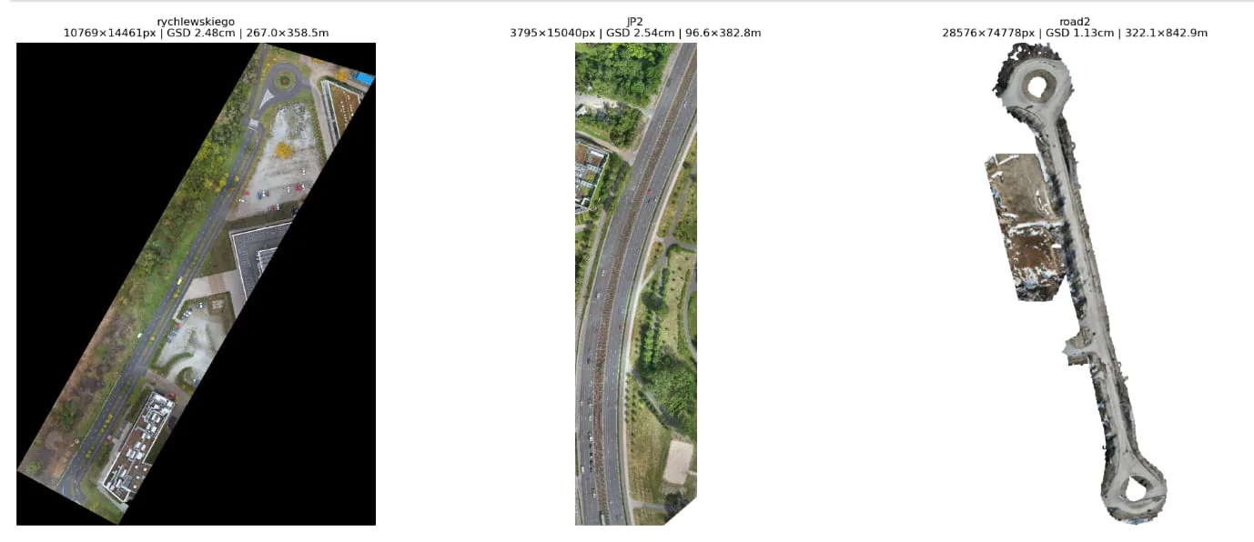
| Scene | GSD | Area | Detections | Mean confidence |
|---|---|---|---|---|
| rychlewskiego | 2.48 cm/px | 267 × 359 m | 104 | 0.25 |
| JP2 | 2.54 cm/px | 97 × 383 m | 49 | 0.30 |
| road2 | 1.13 cm/px | 322 × 843 m | 2,201 | 0.30 |
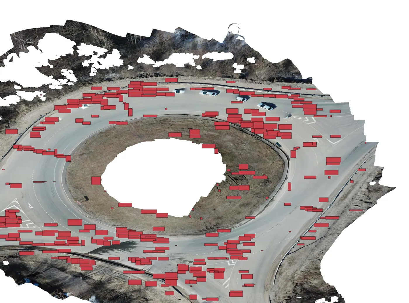
The pipeline found all six defect classes on the largest scene. Oblique cracks dominate every scene, and on road2 they cluster around a roundabout, where turning traffic stresses the surface at an angle. The detections loaded into QGIS on top of the source rasters landed on visible pavement damage, with the coordinate system matching the source file.
The honest number
Mean confidence on these orthophotos is 0.25 to 0.30. On the benchmark test set it is above 0.9. That gap is the domain shift made visible: different region, different height, different camera.
I kept the confidence threshold at 0.10 on purpose. The intended workflow is an engineer reviewing detections in GIS, so a missed crack costs more than a false one that takes two seconds to dismiss. Raising the threshold to 0.25 would drop about 40% of detections in one scene, and without ground truth I couldn't show that it would remove more wrong boxes than right ones.
Roadster: a tool instead of notebooks
Research code lives in notebooks, and nobody who plans road repairs will open one. So the last part of the thesis wrapped everything in Roadster, a small local app: a Flask server with a single-page front end.
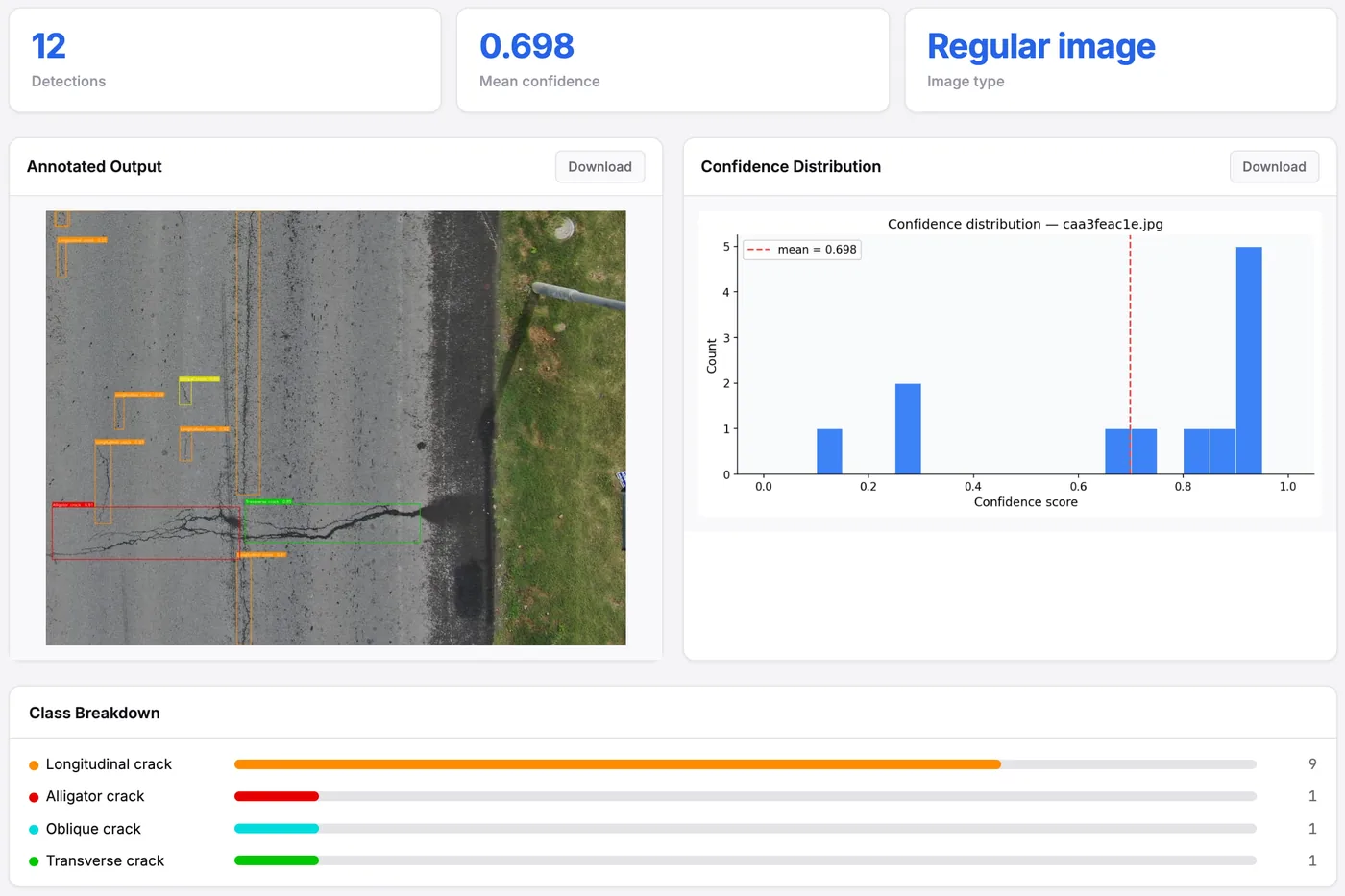
You pick one of the five trained models, drop in a photo or a GeoTIFF, set the confidence and IoU thresholds with sliders, and get the annotated image, a per-class breakdown, a confidence histogram and the CSV and GeoJSON files to download. It detects whether a file is an orthophoto by checking for a coordinate system and a real affine transform, and runs the tiling pipeline when it is. Inference runs in a background thread, and the page polls for progress.
Limits, plainly
- No ground truth on the field orthophotos. I can show the detections line up with real damage in QGIS, but I can't give precision or recall on them. Labelling even part of one scene is the most valuable next step.
- One architecture, one training dataset. The ranking of the three axes might not hold for another model or another country's roads.
- The resolution effect isn't isolated, as above.
- Large defects can be split across tiles in a way cross-tile NMS can't merge back.
- The model has no idea what a road is. In urban scenes it sometimes fires on rooftops or courtyards whose texture looks like worn asphalt. Clipping the orthophoto to OpenStreetMap road polygons before tiling would fix most of that without touching the model.
What I took away
The benchmark number was the easy part. The real work was everything between a model file and a row in an engineer's spreadsheet: matching scale, stitching tiles back together, getting coordinates right, and choosing a threshold for the person who reviews the output rather than for a leaderboard. That is the same lesson as in data platforms. The model, like a pipeline, is only as useful as the place its output lands.
The papers
- A. Mustafa, M. Yu. Kataev, D. S. Efremenko. Detection of Road Defects from Unmanned Aerial Vehicles Using Machine Learning. Light & Engineering 34(3), pp. 4 to 12, 2026.
- A. Mustafa, M. Yu. Kataev, D. S. Efremenko. Structured Training Ablation and GSD-Adaptive Orthophoto Inference for UAV-Based Pavement Defect Detection with YOLO26. Moscow University Physics Bulletin, 2026, in press. Presented at DLCP 2026.
Abstracts and BibTeX are in the research section of the home page, and everything I publish is on my Google Scholar profile. The charts and figures here are my own, from the thesis work behind both papers.